Longer introduction
Let’s explore the methods and attributes available in the ERDDAP object? Note that we can either use the short server key (NGDAC) or the full URL. For a list of the short keys check erddapy.servers.
[1]:
from erddapy import ERDDAP

server = "https://gliders.ioos.us/erddap"
e = ERDDAP(server=server)

[method for method in dir(e) if not method.startswith("_")]
[1]:
['auth',
 'constraints',
 'dataset_id',
 'dim_names',
 'download_file',
 'get_categorize_url',
 'get_download_url',
 'get_info_url',
 'get_search_url',
 'get_var_by_attr',
 'griddap_initialize',
 'protocol',
 'requests_kwargs',
 'response',
 'server',
 'server_functions',
 'to_iris',
 'to_ncCF',
 'to_pandas',
 'to_xarray',
 'variables']
All the methods prefixed with _get__ will return a valid ERDDAP URL for the requested response and options. For example, searching for all datasets available.
[2]:
url = e.get_search_url(search_for="all", response="html")

print(url)
https://gliders.ioos.us/erddap/search/advanced.html?page=1&itemsPerPage=1000000&protocol=(ANY)&cdm_data_type=(ANY)&institution=(ANY)&ioos_category=(ANY)&keywords=(ANY)&long_name=(ANY)&standard_name=(ANY)&variableName=(ANY)&minLon=(ANY)&maxLon=(ANY)&minLat=(ANY)&maxLat=(ANY)&minTime=&maxTime=&searchFor=all
There are many responses available, see the docs for griddap and tabledap respectively. The most useful ones for Pythonistas are the .csv and .nc that can be read with pandas and netCDF4-python respectively.
Let’s load the csv response directly with pandas.
[3]:
import pandas as pd

url = e.get_search_url(search_for="whoi", response="csv")

df = pd.read_csv(url)
print(
    f"We have {len(set(df['tabledap'].dropna()))} "
    f"tabledap, {len(set(df['griddap'].dropna()))} "
    f"griddap, and {len(set(df['wms'].dropna()))} wms endpoints.",
)
We have 479 tabledap, 0 griddap, and 0 wms endpoints.
We can refine our search by providing some constraints.
Let’s narrow the search area, time span, and look for sea_water_temperature.
[4]:
kw = {
    "standard_name": "sea_water_temperature",
    "min_lon": -72.0,
    "max_lon": -69.0,
    "min_lat": 38.0,
    "max_lat": 41.0,
    "min_time": "2016-07-10T00:00:00Z",
    "max_time": "2017-02-10T00:00:00Z",
    "cdm_data_type": "trajectoryprofile",
}


search_url = e.get_search_url(response="html", **kw)
print(search_url)
https://gliders.ioos.us/erddap/search/advanced.html?page=1&itemsPerPage=1000000&protocol=(ANY)&cdm_data_type=trajectoryprofile&institution=(ANY)&ioos_category=(ANY)&keywords=(ANY)&long_name=(ANY)&standard_name=sea_water_temperature&variableName=(ANY)&minLon=-72.0&maxLon=-69.0&minLat=38.0&maxLat=41.0&minTime=1468108800.0&maxTime=1486684800.0
The search form was populated with the constraints we provided. Click on the URL above to see how that looks on the server HTML form page.
Changing the response from html to csv we load it in a data frame.
[5]:
search_url = e.get_search_url(response="csv", **kw)
search = pd.read_csv(search_url)
gliders = search["Dataset ID"].to_numpy()

gliders_list = "\n".join(gliders)
print(f"Found {len(gliders)} Glider Datasets:\n{gliders_list}")
Found 19 Glider Datasets:
blue-20160818T1448
cp_335-20170116T1459-delayed
cp_336-20160809T1354-delayed
cp_336-20161011T0058-delayed
cp_336-20170116T1254-delayed
cp_339-20170116T2353-delayed
cp_340-20160809T0621-delayed
cp_374-20140416T1634-delayed
cp_374-20150509T1256-delayed
cp_374-20160529T0026-delayed
cp_376-20160527T2050-delayed
cp_380-20161011T2046-delayed
cp_387-20160404T1858-delayed
cp_388-20160809T1406-delayed
cp_388-20170116T1324-delayed
cp_389-20161011T2040-delayed
silbo-20160413T1534
sp022-20170209T1616
whoi_406-20160902T1700
Now that we know the Dataset ID we can explore their metadata with the get_info_url method.
[6]:
glider = gliders[-1]

info_url = e.get_info_url(dataset_id=glider, response="html")

print(info_url)
https://gliders.ioos.us/erddap/info/whoi_406-20160902T1700/index.html
You can follow the URL above and check this particular dataset_id index page on the server.
We can manipulate the metadata and find the variables that have the cdm_profile_variables attribute using the csv response.
[7]:
info_url = e.get_info_url(dataset_id=glider, response="csv")

info = pd.read_csv(info_url)
info.head()
[7]:
| Row Type | Variable Name | Attribute Name | Data Type | Value | |
|---|---|---|---|---|---|
| 0 | attribute | NC_GLOBAL | acknowledgment | String | This deployment supported by NOAA through the ... |
| 1 | attribute | NC_GLOBAL | cdm_data_type | String | TrajectoryProfile |
| 2 | attribute | NC_GLOBAL | cdm_profile_variables | String | time_uv,lat_uv,lon_uv,u,v,profile_id,time,lati... |
| 3 | attribute | NC_GLOBAL | cdm_trajectory_variables | String | trajectory,wmo_id |
| 4 | attribute | NC_GLOBAL | comment | String | Glider operatored by Woods Hole Oceanographic ... |
[8]:
"".join(info.loc[info["Attribute Name"] == "cdm_profile_variables", "Value"])
[8]:
'time_uv,lat_uv,lon_uv,u,v,profile_id,time,latitude,longitude'
Selecting variables by theirs attributes is such a common operation that erddapy brings its own method to simplify this task.
The get_var_by_attr method was inspired by netCDF4-python’s get_variables_by_attributes. However, because erddapy operates on remote serves, it will return the variable names instead of the actual data.
We ca check what is/are the variable(s) associated with the standard_name used in the search.
Note that get_var_by_attr caches the last response in case the user needs to make multiple requests. (See the execution times below.)
[9]:
%%time

# First request can be slow.
e.get_var_by_attr(
    dataset_id="whoi_406-20160902T1700",
    standard_name="sea_water_temperature",
)
CPU times: user 74.3 ms, sys: 4.1 ms, total: 78.4 ms
Wall time: 130 ms
[9]:
['temperature']
[10]:
%%time

# Second request on dataset_id will be faster.
e.get_var_by_attr(
    dataset_id="whoi_406-20160902T1700",
    standard_name="sea_water_practical_salinity",
)
CPU times: user 28 μs, sys: 3 μs, total: 31 μs
Wall time: 33.9 μs
[10]:
['salinity']
Another way to browse datasets is via the categorize URL. In the example below we can get all the standard_names available in the dataset with a single request.
[11]:
url = e.get_categorize_url(categorize_by="standard_name", response="csv")

pd.read_csv(url)["Category"]
[11]:
0                                                  _null
1                                 aggregate_quality_flag
2                                               altitude
3                                            backscatter
4                 barotropic_eastward_sea_water_velocity
                             ...
141    volume_fraction_of_oxygen_in_sea_water_status_...
142    volume_scattering_coefficient_of_radiative_flu...
143    volume_scattering_function_of_radiative_flux_i...
144                              water_velocity_eastward
145                             water_velocity_northward
Name: Category, Length: 146, dtype: str
We can also pass a value to filter the categorize results.
[12]:
url = e.get_categorize_url(
    categorize_by="institution",
    value="woods_hole_oceanographic_institution",
    response="csv",
)

df = pd.read_csv(url)
whoi_gliders = df.loc[~df["tabledap"].isna(), "Dataset ID"].tolist()
whoi_gliders
[12]:
['sp007-20170427T1652',
 'sp007-20200618T1527',
 'sp007-20210818T1548',
 'sp007-20220330T1436',
 'sp007-20230208T1524',
 'sp007-20230614T1428',
 'sp007-20240425T1202',
 'sp007-20250418T1600',
 'sp010-20150409T1524',
 'sp010-20170707T1647',
 'sp010-20180620T1455',
 'sp022-20170209T1616',
 'sp022-20170802T1414',
 'sp022-20180124T1514',
 'sp022-20180422T1229',
 'sp022-20180912T1553',
 'sp022-20201113T1549',
 'sp055-20150716T1359',
 'sp062-20171116T1557',
 'sp062-20190201T1350',
 'sp062-20190925T1538',
 'sp062-20200227T1647',
 'sp062-20200824T1618',
 'sp062-20210624T1335',
 'sp062-20211014T1515',
 'sp062-20220623T1419',
 'sp062-20230316T1547',
 'sp062-20230823T1452',
 'sp062-20240410T1536',
 'sp062-20250702T1440',
 'sp065-20151001T1507',
 'sp065-20180310T1828',
 'sp065-20181015T1349',
 'sp065-20190517T1530',
 'sp065-20191120T1543',
 'sp065-20200506T1709',
 'sp065-20210616T1430',
 'sp065-20220202T1520',
 'sp065-20221116T1552',
 'sp065-20230414T1618',
 'sp065-20240214T1520',
 'sp065-20240617T1658',
 'sp065-20250115T1528',
 'sp066-20151217T1624',
 'sp066-20160818T1505',
 'sp066-20170416T1744',
 'sp066-20171129T1616',
 'sp066-20180629T1411',
 'sp066-20190301T1640',
 'sp066-20190724T1532',
 'sp066-20200123T1630',
 'sp066-20200824T1631',
 'sp066-20210624T1332',
 'sp066-20221012T1417',
 'sp066-20230316T1546',
 'sp066-20231018T1432',
 'sp066-20240425T1204',
 'sp066-20241106T1639',
 'sp069-20170907T1531',
 'sp069-20180411T1516',
 'sp069-20181109T1607',
 'sp069-20200319T1317',
 'sp069-20210408T1555',
 'sp069-20230507T1437',
 'sp069-20230731T1323',
 'sp069-20240703T1534',
 'sp069-20250404T1341',
 'sp069-20250728T1600',
 'sp070-20220824T1510',
 'sp070-20230316T1541',
 'sp070-20240912T1432',
 'sp071-20211215T2041',
 'sp071-20220602T1317',
 'sp071-20230507T1431',
 'sp071-20231220T1541',
 'sp071-20240617T1659',
 'sp071-20250501T1427',
 'sp209-20251105T1645',
 'sp210-20260205T1802',
 'sp211-20260603T1615',
 'sp212-20260107T1615',
 'sp213-20260317T1523',
 'whoi_406-20160902T1700']
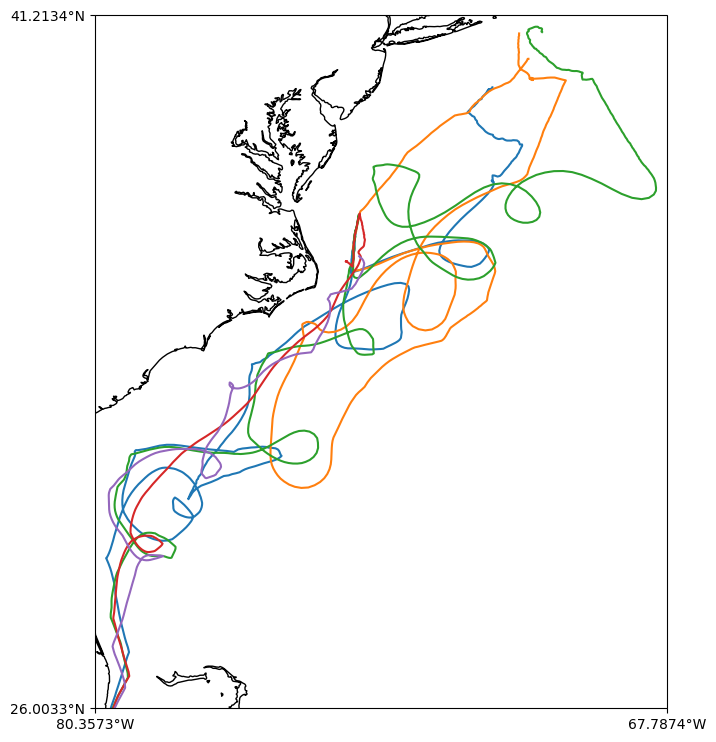
Let’s create a map of some WHOI gliders tracks.
We are downloading a lot of data! Note that we will use joblib to parallelize the for loop and get the data faster and we will limit to the first 5 gliders.
[13]:
import multiprocessing

from joblib import Parallel, delayed

from erddapy.core import get_download_url, to_pandas


def request_whoi(dataset_id):
    variables = ["longitude", "latitude", "temperature", "salinity"]
    url = get_download_url(
        server,
        dataset_id=dataset_id,
        protocol="tabledap",
        variables=variables,
        response="csv",
    )
    # Drop units in the first line and NaNs.
    df = to_pandas(url, pandas_kwargs={"skiprows": (1,)}).dropna()
    return (dataset_id, df)


num_cores = multiprocessing.cpu_count()
downloads = Parallel(n_jobs=num_cores)(
    delayed(request_whoi)(dataset_id) for dataset_id in whoi_gliders[:5]
)

dfs = dict(downloads)
Finally let’s see some figures!
[14]:
import cartopy.crs as ccrs
import matplotlib.pyplot as plt
from cartopy.mpl.ticker import LatitudeFormatter, LongitudeFormatter


def make_map():
    fig, ax = plt.subplots(
        figsize=(9, 9),
        subplot_kw={"projection": ccrs.PlateCarree()},
    )
    ax.coastlines(resolution="10m")
    lon_formatter = LongitudeFormatter(zero_direction_label=True)
    lat_formatter = LatitudeFormatter()
    ax.xaxis.set_major_formatter(lon_formatter)
    ax.yaxis.set_major_formatter(lat_formatter)

    return fig, ax


fig, ax = make_map()
lons, lats = [], []
for df in dfs.values():
    lon, lat = df["longitude"], df["latitude"]
    lons.extend(lon.array)
    lats.extend(lat.array)
    ax.plot(lon, lat)

dx = dy = 0.25
extent = min(lons) - dx, max(lons) + dx, min(lats) + dy, max(lats) + dy
ax.set_extent(extent)

ax.set_xticks([extent[0], extent[1]], crs=ccrs.PlateCarree())
ax.set_yticks([extent[2], extent[3]], crs=ccrs.PlateCarree());

[15]:
def glider_scatter(df, ax):
    ax.scatter(df["temperature"], df["salinity"], s=10, alpha=0.25)


fig, ax = plt.subplots(figsize=(9, 9))
ax.set_ylabel("salinity")
ax.set_xlabel("temperature")
ax.grid(True)

for df in dfs.values():
    glider_scatter(df, ax)

ax.axis([5.5, 30, 30, 38])
[15]:
(np.float64(5.5), np.float64(30.0), np.float64(30.0), np.float64(38.0))
[16]:
e.dataset_id = "whoi_406-20160902T1700"
e.protocol = "tabledap"
e.variables = [
    "depth",
    "latitude",
    "longitude",
    "salinity",
    "temperature",
    "time",
]

e.constraints = {
    "time>=": "2016-09-03T00:00:00Z",
    "time<=": "2017-02-10T00:00:00Z",
    "latitude>=": 38.0,
    "latitude<=": 41.0,
    "longitude>=": -72.0,
    "longitude<=": -69.0,
}


df = e.to_pandas(
    index_col="time (UTC)",
    parse_dates=True,
).dropna()
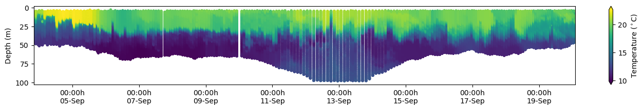
[17]:
import matplotlib.dates as mdates

fig, ax = plt.subplots(figsize=(17, 2))
cs = ax.scatter(
    df.index,
    df["depth (m)"],
    s=15,
    c=df["temperature (Celsius)"],
    marker="o",
    edgecolor="none",
)

ax.invert_yaxis()
ax.set_xlim(df.index[0], df.index[-1])
xfmt = mdates.DateFormatter("%H:%Mh\n%d-%b")
ax.xaxis.set_major_formatter(xfmt)

cbar = fig.colorbar(cs, orientation="vertical", extend="both")
cbar.ax.set_ylabel(r"Temperature ($^\circ$C)")
ax.set_ylabel("Depth (m)")
[17]:
Text(0, 0.5, 'Depth (m)')