Near real-time HF-Radar currents in the proximity of the Deepwater Horizon site

Near real-time HF-Radar currents in the proximity of the Deepwater Horizon site#

Created: 2017-07-25

Updated: 2026-05-01

The explosion on the Deepwater Horizon (DWH) tragically killed 11 people, and resulted in one of the largest marine oil spills in history. One of the first questions when there is such a tragedy is: where will the oil go if that happened today?

In order the help answer that question one can use near real time currents from the HF-Radar sites near the incident.

First let’s start with the HF-Radar site, where one can browse the available data interactively. Below we show an IFrame for the site.

In this notebook we will demonstrate how to obtain such data programmatically.

(For more information on the DWH see http://response.restoration.noaa.gov/oil-and-chemical-spills/significant-incidents/deepwater-horizon-oil-spill.)

from IPython.display import IFrame

url = "https://hfradar.ioos.us/hfrnet/"

IFrame(
    src=url,
    width=750,
    height=450,
)

The interactive interface is handy for exploration but we usually need to download “mechanically” in order to use them in our analysis, plots, or for downloading time-series.

One way to achieve that is to use an OPeNDAP client, here Python’s xarray, and explore the endpoints directly. The NCEI hfradar catalog is organized in folders and subfolders by year, month, region and then individual files that contains the datetime info and data resolution. The regions are:

USWC → West Coast
USHI → Hawaii
USEGC → US East and Gulf Coasts
PRVI → Puerto Rico/Virgin Islands
AKNS → Alaska North Slope
GLNA → Great Lakes North America
GAK → Gulf of Alaska

Note that the region folders and file names can change from year to year. We will download data around 2017-07-25, the original data when this notebooks was first posted.

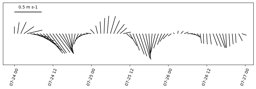
How about extracting a day time-series from the dataset and then averaged around the area of interest?

dx = dy = 2.25  # Area around the point of interest.
center = -87.373643, 29.061888  # Point of interest.

dsr = ds.sel(
    lon=(ds.lon < center[0] + dx) & (ds.lon > center[0] - dx),
    lat=(ds.lat < center[1] + dy) & (ds.lat > center[1] - dy),
)

avg = dsr.mean(dim=["lon", "lat"])
time = avg["time"].to_index().to_pydatetime()

Now all we have to do is mask the missing data with NaNs and average over the area.

import numpy.ma as ma

v = avg["v"].data
u = avg["u"].data

u = ma.masked_invalid(u)
v = ma.masked_invalid(v)

import matplotlib.pyplot as plt
from oceans.plotting import stick_plot

fig, ax = plt.subplots(figsize=(11, 2.75))

q = stick_plot(time, u, v, ax=ax)

ref = 0.5
qk = plt.quiverkey(
    q,
    0.1,
    0.85,
    ref,
    "{} {}".format(ref, ds["u"].units),
    labelpos="N",
    coordinates="axes",
)

_ = plt.xticks(rotation=70)

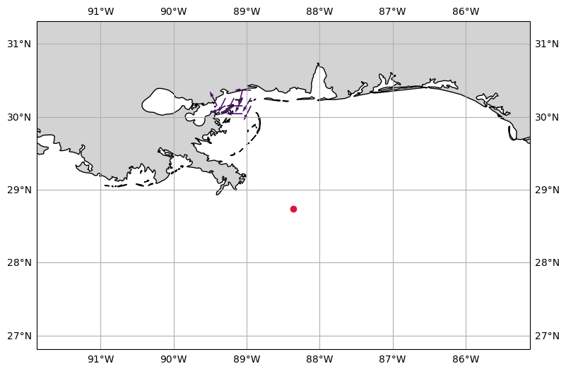
../../../_images/faca0aa234c67101f00c29de2317c3690a84cafe08dc9cc843c8d67148c23576.png

To close this post let’s us reproduce the HF radar image from the interactive site using yesterday’s data and the NRT endpoint from NDBC.

from datetime import date, timedelta

ds = xr.open_dataset(
    "https://dods.ndbc.noaa.gov/thredds/dodsC/hfradar_usegc_6km_25hravg"
)
yesterday = date.today() - timedelta(days=1)
dsy = ds.sel(time=yesterday, method="nearest")

Now that we singled out the date and and time we want the data, we trigger the download by accessing the data with xarray’s .data property.

u = dsy["u_mean"].data
v = dsy["v_mean"].data

lon = dsy.coords["lon"].data
lat = dsy.coords["lat"].data
time = dsy.coords["time"].data

The cell below computes the speed from the velocity. We can use the speed computation to color code the vectors. Note that we re-create the vector velocity preserving the direction but using intensity of 1. (The same visualization technique used in the HF radar DAC.)

import numpy as np
from oceans.ocfis import spdir2uv, uv2spdir

angle, speed = uv2spdir(u, v)
us, vs = spdir2uv(np.ones_like(speed), angle, deg=True)

Now we can create a matplotlib figure displaying the data.

import cartopy.crs as ccrs
from cartopy import feature
from cartopy.mpl.gridliner import LATITUDE_FORMATTER, LONGITUDE_FORMATTER

LAND = feature.NaturalEarthFeature(
    "physical", "land", "10m", edgecolor="face", facecolor="lightgray"
)

sub = 2
bbox = lon.min(), lon.max(), lat.min(), lat.max()

fig, ax = plt.subplots(figsize=(9, 9), subplot_kw=dict(projection=ccrs.PlateCarree()))


ax.set_extent([center[0] - dx - dx, center[0] + dx, center[1] - dy, center[1] + dy])
vmin, vmax = np.nanmin(speed[::sub, ::sub]), np.nanmax(speed[::sub, ::sub])
speed_clipped = np.clip(speed[::sub, ::sub], 0, 0.65)
ax.quiver(
    lon[::sub],
    lat[::sub],
    us[::sub, ::sub],
    vs[::sub, ::sub],
    speed_clipped,
    scale=30,
)

# Deepwater Horizon site.
ax.plot(-88.365997, 28.736628, marker="o", color="crimson")
gl = ax.gridlines(draw_labels=True)
gl.xlabels_top = gl.ylabels_right = False
gl.xformatter = LONGITUDE_FORMATTER
gl.yformatter = LATITUDE_FORMATTER

feature = ax.add_feature(LAND, zorder=0, edgecolor="black")

../../../_images/a7d98db48c3df1f1be5dcba640def3b68052db3954137db7808079c7efca68b6.png